Introduction to SDF
Signed Distance Field (SDF)
Signed Distance Field (SDF)1 is a mathematical function or data structure used to represent shapes. In 2D or 3D space, it assigns each point a signed distance value, which represents the distance to the nearest surface (or boundary), with the sign distinguishing between inside and outside:
- Positive value: The point is outside the shape, and the value indicates the nearest distance to the surface.
- Negative value: The point is inside the shape, and the absolute value indicates the nearest distance to the surface.
- Zero: The point lies exactly on the surface of the shape.
Formally, for a point $x$ in space, an SDF can be defined as:
$$ f(x) = \begin{cases} d(x, \partial\Omega), & \text{if } x \in \Omega \\ -d(x, \partial\Omega), & \text{if } x \notin \Omega \\ 0, & \text{if } x \in \partial\Omega \end{cases} $$
where $\Omega$ denotes the interior of the object, $\partial\Omega$ its boundary, and $d(x, \partial\Omega)$ the minimum distance from $x$ to the boundary.
GitHub Repository
If you want to check out the final code that generates SDF images, you can find it in the GitHub repo2: cronrpc/Signed-Distance-Field-2D-Generator
Applications
The definition above may sound abstract, so let’s look at some practical applications:
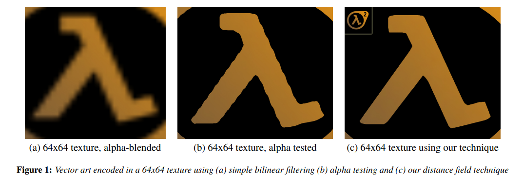
- Font rendering (Valve’s SDF font technology3; Unity’s TMP fonts use SDF as well).
Surface intersection in ray tracing
Stylized shadows, clouds, and similar effects
In general, any scenario involving continuous transitions can potentially leverage SDF techniques.
2D SDF Generation Algorithms
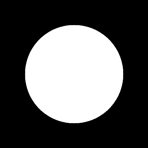
For a grayscale image where white represents the object and black represents the background, how do we generate an SDF image?
Brute-Force Evaluation
The simplest approach is brute force:
- Identify all boundary pixels (a white pixel with at least one black neighbor).
- For every pixel, compute the nearest distance to the boundary set.
- Assign a positive or negative sign based on whether the pixel itself is inside (white) or outside (black).
If the total number of pixels is $n$, the complexity is $O(n^2)$.
# generator_sdf.py
import sys
import math
from PIL import Image
import numpy as np

def generate_sdf(input_path, output_path):
    # Read grayscale image (0–255)
    img = Image.open(input_path).convert("L")
    w, h = img.size
    pixels = np.array(img)

    # Step 1: Find boundary pixels
    boundary_points = []
    for y in range(h):
        for x in range(w):
            if pixels[y, x] > 127:
                neighbors = [
                    (nx, ny)
                    for nx in (x - 1, x, x + 1)
                    for ny in (y - 1, y, y + 1)
                    if 0 <= nx < w and 0 <= ny < h and not (nx == x and ny == y)
                ]
                for nx, ny in neighbors:
                    if pixels[ny, nx] <= 127:
                        boundary_points.append((x, y))
                        break

    # Step 2 & 3: Compute SDF
    sdf = np.zeros((h, w), dtype=np.float32)
    for y in range(h):
        for x in range(w):
            min_dist = float("inf")
            for bx, by in boundary_points:
                dist = math.sqrt((x - bx) ** 2 + (y - by) ** 2)
                if dist < min_dist:
                    min_dist = dist
            # Negative for background
            if pixels[y, x] <= 127:
                min_dist = -min_dist
            sdf[y, x] = min_dist

    # Normalize to 0–255
    max_dist = np.max(np.abs(sdf))
    sdf_normalized = ((sdf / max_dist) + 1) * 127.5
    sdf_img = Image.fromarray(np.clip(sdf_normalized, 0, 255).astype(np.uint8))
    sdf_img.save(output_path)
    print(f"SDF saved to {output_path}")

if __name__ == "__main__":
    if len(sys.argv) != 3:
        print("Example: python generator_sdf.py test.png test_sdf.png")
        sys.exit(1)
    generate_sdf(sys.argv[1], sys.argv[2])
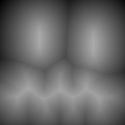
Generated result:
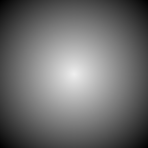
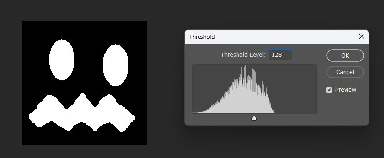
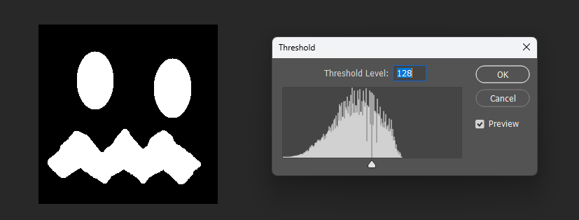
By adjusting the display threshold in Photoshop, we can observe the SDF transitions:
Similarly, for a square, its SDF exhibits right-angle contours inside and circular contours outside:
8-Neighborhood Euclidean Approximation
A metric space 4 is an abstract mathematical framework that defines the notion of “distance.” It consists of a set $X$ and a distance function
$$ d : X \times X \to \mathbb{R} $$
which must satisfy the following four conditions:
- Non-negativity: Distance is always non-negative.
- Identity: Distance is zero if and only if the two points are identical.
- Symmetry: The distance from $x$ to $y$ is the same as from $y$ to $x$.
- Triangle inequality: Taking a detour should never be shorter than going directly.
$$ d(x, z) \le d(x, y) + d(y, z) $$
For example, in the continuous 2D plane, the Euclidean distance
$$ d(P, Q) = \sqrt{(x_P - x_Q)^2 + (y_P - y_Q)^2} $$
is a typical metric.
In the figure below, the blue, red, and yellow lines all represent the same length, while the green line is the shorter Euclidean distance.
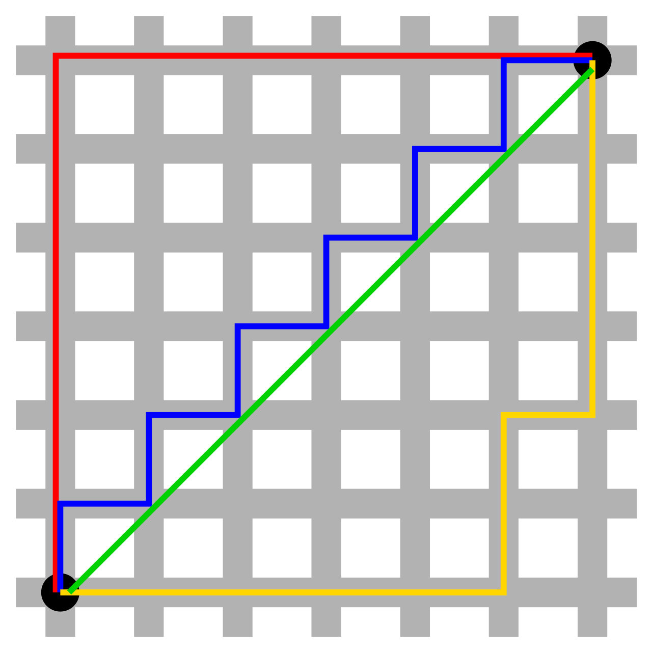
However, in digital image processing or raster maps, our points are discrete pixels. While distances can be computed using the Euclidean formula, doing so requires many square root operations, which are computationally expensive.
To improve efficiency, we often use the 8-neighborhood Euclidean approximation:
- 8-neighborhood: Each pixel is considered adjacent to the 8 nearest pixels — horizontally, vertically, and diagonally.
- The approximate Euclidean distance is then defined as:
$$ d_{8}(p, q) \approx \max(\Delta x, \Delta y) + (\sqrt{2} - 1) \cdot \min(\Delta x, \Delta y) $$
where $\Delta x = |x_p - x_q|$,$\Delta y = |y_p - y_q|$。
For example, in the figure below, the red path represents the 8-neighborhood Euclidean approximation, while the blue line is the true Euclidean distance.
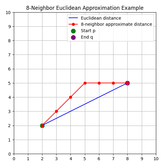
This method avoids costly square root operations, and within the 8-neighborhood its error compared to the true Euclidean distance is small. Therefore, it is widely used in pathfinding (A*, Dijkstra), distance transforms, and morphological image processing.
8SSEDT
This algorithm is based on Lisapple’s 8SSEDT5.
In the previous section, we introduced the 8-neighborhood Euclidean approximation. In fact, for each node in the grid, its distance can be expressed recursively as:
$$ f(x, y) = \min_{\substack{dx, dy \in {-1,0,1} \ (dx, dy) \neq (0,0)}} \Big( f(x+dx, y+dy) + d(dx, dy) \Big) $$
where $d(dx, dy)$ is the cost of moving from neighbor $(x+dx, y+dy)$ to $(x, y)$, usually defined as:
$$ d(dx, dy) = \begin{cases} 1, & \text{where } |dx| + |dy| = 1 \quad (\text{horizontal or vertical neighbor})\\ \sqrt{2}, & \text{where } |dx| + |dy| = 2 \quad (\text{diagonal neighbor}) \end{cases} $$
Here, $dx$ and $dy$ can each be $-1, 0, 1$, but not both zero, since that would not be a neighbor.
If we label the neighbors:
[#1][#2][#3]
[#4][ x][#5]
[#6][#7][#8]
The path between any two points $x$ and $y$ must be composed of one of the following four combinations:
1,2,4

2,3,5

4,6,7

5,7,8
Thus, propagating from the top-left to the bottom-right covers the $1,2,4$ case, meaning that at most four full passes over the grid are needed to compute all values.
An optimization, inspired by Signed Distance Fields6, chooses the following four traversal paths instead:
   - - - >
| [?][?][?]
| [?][x][ ]
v [ ][ ][ ]

   < - - -
| [ ][ ][ ]
| [ ][x][?]
v [ ][ ][ ]

   < - - -
^ [ ][ ][ ]
| [ ][x][?]
| [?][?][?]

   - - - >
^ [ ][ ][ ]
| [?][x][ ]
| [ ][ ][ ]
Here is the Python implementation:
- Strictly speaking, the following code computes the true Euclidean distance, not the 8-neighborhood approximation.
- It only borrows the idea of 8 possible directions of movement.
import sys
import os
import numpy as np
from PIL import Image

INF = 9999

def dist_sq(dx, dy):
    return dx*dx + dy*dy

def compare(grid, p, x, y, ox, oy, width, height):
    nx = x + ox
    ny = y + oy
    if 0 <= nx < width and 0 <= ny < height:
        other_dx, other_dy = grid[ny, nx]
    else:
        other_dx, other_dy = INF, INF
    other_dx += ox
    other_dy += oy
    if dist_sq(other_dx, other_dy) < dist_sq(*p):
        p = (other_dx, other_dy)
    return p

def generate_sdf(grid):
    height, width, _ = grid.shape
    # Pass 0
    for y in range(height):
        for x in range(width):
            p = tuple(grid[y, x])
            p = compare(grid, p, x, y, -1,  0, width, height)
            p = compare(grid, p, x, y,  0, -1, width, height)
            p = compare(grid, p, x, y, -1, -1, width, height)
            p = compare(grid, p, x, y,  1, -1, width, height)
            grid[y, x] = p
        for x in range(width-1, -1, -1):
            p = tuple(grid[y, x])
            p = compare(grid, p, x, y, 1, 0, width, height)
            grid[y, x] = p

    # Pass 1
    for y in range(height-1, -1, -1):
        for x in range(width-1, -1, -1):
            p = tuple(grid[y, x])
            p = compare(grid, p, x, y,  1,  0, width, height)
            p = compare(grid, p, x, y,  0,  1, width, height)
            p = compare(grid, p, x, y, -1,  1, width, height)
            p = compare(grid, p, x, y,  1,  1, width, height)
            grid[y, x] = p
        for x in range(width):
            p = tuple(grid[y, x])
            p = compare(grid, p, x, y, -1, 0, width, height)
            grid[y, x] = p

def load_image_binary(path, threshold=128):
    im = Image.open(path).convert('L')
    arr = np.array(im, dtype=np.uint8)
    inside = arr < threshold
    return inside, im

def save_signed_sdf_image(signed, out_path):
    max_dist = np.max(np.abs(signed))
    if max_dist == 0:
        sdf_normalized = np.full_like(signed, 128.0)
    else:
        sdf_normalized = ((signed / max_dist) + 1.0) * 128.0
    sdf_normalized = np.clip(sdf_normalized, 0, 255).astype(np.uint8)
    out = Image.fromarray(sdf_normalized, mode='L')
    out.save(out_path)

def main():
    if len(sys.argv) < 2:
        print("Usage: python 8ssedt.py input.png")
        sys.exit(1)

    in_path = sys.argv[1]
    if not os.path.exists(in_path):
        print("File not found:", in_path)
        sys.exit(1)

    inside, im = load_image_binary(in_path)
    h, w = inside.shape
    empty = (INF, INF)
    zero = (0, 0)

    # two grids: inside distances and outside distances
    grid1 = np.zeros((h, w, 2), dtype=int)
    grid2 = np.zeros((h, w, 2), dtype=int)

    for y in range(h):
        for x in range(w):
            if inside[y, x]:
                grid1[y, x] = zero
                grid2[y, x] = empty
            else:
                grid1[y, x] = empty
                grid2[y, x] = zero

    generate_sdf(grid1)
    generate_sdf(grid2)

    dist1 = np.sqrt(grid1[:, :, 0]**2 + grid1[:, :, 1]**2)
    dist2 = np.sqrt(grid2[:, :, 0]**2 + grid2[:, :, 1]**2)
    signed = dist1 - dist2

    base, ext = os.path.splitext(in_path)
    out_path = base + "_8ssedt.png"
    save_signed_sdf_image(signed, out_path)
    print("Saved:", out_path)

if __name__ == "__main__":
    main()
We can test it on this input image:

After running the script, we get:
Visualized in Photoshop with different thresholds:
Correct 8SSEDT
As noted in 7, the issue with binary black-and-white images is that for pixels near the boundary, the true distance to the boundary should actually be only half a pixel.
Ignoring this half-pixel offset leads to small inaccuracies near boundaries. The fix is to add only half the step size when the neighboring pixel is on the boundary.
import sys
import os
import math
import numpy as np
from PIL import Image

FIX = True

INF = 9999

def dist_sq(dx, dy):
    return dx*dx + dy*dy

def compare(grid, p, x, y, ox, oy, width, height):
    nx = x + ox
    ny = y + oy
    if 0 <= nx < width and 0 <= ny < height:
        other_dx, other_dy = grid[ny, nx]
    else:
        other_dx, other_dy = INF, INF

    if FIX:
        if other_dx != 0 or other_dy != 0:
            ox *= 2
            oy *= 2

    other_dx += ox
    other_dy += oy
    if dist_sq(other_dx, other_dy) < dist_sq(*p):
        p = (other_dx, other_dy)
    return p

def generate_sdf(grid):
    height, width, _ = grid.shape
    # Pass 0
    for y in range(height):
        for x in range(width):
            p = tuple(grid[y, x])
            p = compare(grid, p, x, y, -1,  0, width, height)
            p = compare(grid, p, x, y,  0, -1, width, height)
            p = compare(grid, p, x, y, -1, -1, width, height)
            p = compare(grid, p, x, y,  1, -1, width, height)
            grid[y, x] = p
        for x in range(width-1, -1, -1):
            p = tuple(grid[y, x])
            p = compare(grid, p, x, y, 1, 0, width, height)
            grid[y, x] = p

    # Pass 1
    for y in range(height-1, -1, -1):
        for x in range(width-1, -1, -1):
            p = tuple(grid[y, x])
            p = compare(grid, p, x, y,  1,  0, width, height)
            p = compare(grid, p, x, y,  0,  1, width, height)
            p = compare(grid, p, x, y, -1,  1, width, height)
            p = compare(grid, p, x, y,  1,  1, width, height)
            grid[y, x] = p
        for x in range(width):
            p = tuple(grid[y, x])
            p = compare(grid, p, x, y, -1, 0, width, height)
            grid[y, x] = p

def load_image_binary(path, threshold=128):
    im = Image.open(path).convert('L')
    arr = np.array(im, dtype=np.uint8)
    inside = arr < threshold
    return inside, im

def save_signed_sdf_image(signed, out_path):
    max_dist = np.max(np.abs(signed))
    if max_dist == 0:
        sdf_normalized = np.full_like(signed, 128.0)
    else:
        sdf_normalized = ((signed / max_dist) + 1.0) * 128.0
    sdf_normalized = np.clip(sdf_normalized, 0, 255).astype(np.uint8)
    out = Image.fromarray(sdf_normalized, mode='L')
    out.save(out_path)

def main():
    if len(sys.argv) < 2:
        print("Usage: python 8ssedt.py input.png")
        sys.exit(1)

    in_path = sys.argv[1]
    if not os.path.exists(in_path):
        print("File not found:", in_path)
        sys.exit(1)

    inside, im = load_image_binary(in_path)
    h, w = inside.shape
    empty = (INF, INF)
    zero = (0, 0)

    # two grids: inside distances and outside distances
    grid1 = np.zeros((h, w, 2), dtype=int)
    grid2 = np.zeros((h, w, 2), dtype=int)

    for y in range(h):
        for x in range(w):
            if inside[y, x]:
                grid1[y, x] = zero
                grid2[y, x] = empty
            else:
                grid1[y, x] = empty
                grid2[y, x] = zero

    generate_sdf(grid1)
    generate_sdf(grid2)

    dist1 = np.sqrt(grid1[:, :, 0]**2 + grid1[:, :, 1]**2)
    dist2 = np.sqrt(grid2[:, :, 0]**2 + grid2[:, :, 1]**2)

    if FIX:
        signed = 0.5 * (dist1 - dist2)
    else:
        signed = dist1 - dist2

    base, ext = os.path.splitext(in_path)
    out_path = base + "_8ssedt_correct.png"
    save_signed_sdf_image(signed, out_path)
    print("Saved:", out_path)

if __name__ == "__main__":
    main()
The results look nearly identical to the original:

But when visualized at different thresholds, the corrected version is slightly smoother near boundaries:
Corrected:
Original:
Why Still Use Euclidean Distance?
Consider the approximation formula:
$$ d_8(p,q) = \max(\Delta x,\Delta y) + (\sqrt{2} - 1) \cdot \min(\Delta x,\Delta y) $$
Take two points: $(1,4)$ and $(3,3)$.
计算 $d_8$
$d_8(1,4) = 4 + (\sqrt{2} - 1) \cdot 1 \approx 4 + 0.4142 = 4.4142$
$d_8(3,3) = 3 + (\sqrt{2} - 1) \cdot 3 \approx 3 + 1.2426 = 4.2426$
⇒ $d_8(1,4) > d_8(3,3)$
计算欧几里得距离
$d_E(1,4) = \sqrt{1^2 + 4^2} = \sqrt{17} \approx 4.1231$
$d_E(3,3) = \sqrt{3^2 + 3^2} = \sqrt{18} \approx 4.2426$
⇒ $d_E(1,4) < d_E(3,3)$
This counterexample shows that $d_8$ does not always preserve the same ordering as Euclidean distance. Therefore, we only borrow the 8-neighborhood displacements, but still compute distances using the Euclidean metric.
The scipy.ndimage Library
The previous Python implementation is slow due to nested loops, especially at resolutions like 2048×2048.
scipy.ndimage provides a much faster alternative, as its image processing functions are implemented in C++.
In the following code, we use a fixed scale of 8 (explained later), and output 16-bit grayscale images instead of 8-bit.
import sys
import os
import numpy as np
from PIL import Image
from scipy import ndimage

scale = 8

def load_image_binary(path, threshold=128):
    im = Image.open(path).convert('L')
    arr = np.array(im, dtype=np.uint8)
    inside = arr < threshold
    return inside

def save_sdf_16bit(signed, out_path):
    signed = signed * scale + 32767.5
    signed_uint16 = np.clip(signed, 0, 65535).astype(np.uint16)
    out = Image.fromarray(signed_uint16, mode='I;16')
    out.save(out_path)

def fast_signed_sdf(mask):
    dist_inside = ndimage.distance_transform_edt(mask)
    dist_outside = ndimage.distance_transform_edt(~mask)
    return dist_outside - dist_inside

def main():
    if len(sys.argv) < 2:
        print("Usage: python fast_sdf.py input1.png [input2.png ...]")
        sys.exit(1)

    for in_path in sys.argv[1:]:
        if not os.path.exists(in_path):
            print("File not found:", in_path)
            continue

        inside = load_image_binary(in_path)
        signed = fast_signed_sdf(inside)

        base, _ = os.path.splitext(in_path)
        out_path = base + "_sdf16.png"
        save_sdf_16bit(signed, out_path)
        print(f"Saved SDF to {out_path}")

if __name__ == "__main__":
    main()
16bit 和 scale
Earlier, we normalized distances, but if we want to combine multiple images, the distance units must be consistent (since interpolation between SDFs depends on this).
Furthermore, with large images (e.g., 2048×2048), 8-bit depth (0–255) is insufficient to represent the full range of distances. To avoid truncation artifacts, we use 16-bit PNGs.
For a 2048×2048 image, the maximum possible distance is about $2048 \cdot 1.414 \approx 2896$. Since 16-bit integers can represent up to $\pm32767$, we can safely choose a scale factor of 8 or 10.
scale = 10
# Map to 0–65535, 32767.5 as the boundary
unsigned = signed * scale + 32767.5
unsigned = np.clip(unsigned, 0, 65535).astype(np.uint16)
Composition Algorithms
How to combine SDFs depends on the desired effect.
For example, if we want a subtraction, can we simply subtract the distance fields?
This works at the midpoint, but at the edges the meaning becomes unclear:
# Boolean operations
def sdf_union(d1, d2):
    return np.minimum(d1, d2)  # Union

def sdf_intersection(d1, d2):
    return np.maximum(d1, d2)  # Intersection

def sdf_subtraction(d1, d2):
    return np.maximum(d1, -d2) # A subtract B
These operations essentially define the effect when crossing the threshold boundary.
Interpolation Approach
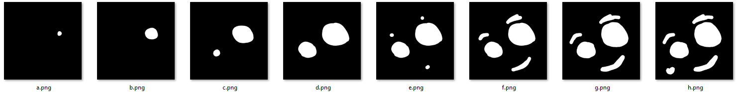
In games, what we often want is this: given two images a and b, at maximum threshold we see a, at minimum threshold we see b.
For three images, the highest threshold shows a, the middle threshold shows b, and the lowest threshold shows c, and so on.
A key requirement is that they must have a containment relationship: $c \supset b \supset a$. Otherwise, the transition cannot be well-defined.
For an arbitrary pixel in a, its distance values in both a and b should be positive (inside).
For a pixel in $b - a$, its distance in a will be negative ($x_a$), and in b positive ($x_b$). Thus, the final SDF value $x_{final}$ is determined by finding the threshold where interpolation between $x_a$ and $x_b$ crosses zero.
For example, if ${sdf}_a = -3$ and ${sdf}b = 3$, then at 8-bit gray, ${x}{final}$ should be 128 — meaning the pixel is lit at thresholds below 128.
So the core idea is: find the zero-crossing point.
Monte Carlo Interpolation
We can approximate the zero point via sampling, as in 8.
Note that pure Python with nested loops is too slow for large images (>2048).
import sys
import numpy as np
from PIL import Image

if len(sys.argv) != 3:
    print("Usage: python compose2.py a.png b.png")
    sys.exit(1)

# Load a 16-bit grayscale image
def load_16bit_gray(path):
    img = Image.open(path)
    arr = np.array(img, dtype=np.uint16)
    return arr

sdf1 = load_16bit_gray(sys.argv[1])
sdf2 = load_16bit_gray(sys.argv[2])

# Ensure dimensions match
if sdf1.shape != sdf2.shape:
    raise ValueError("The two input images must have the same dimensions")

height, width = sdf1.shape
output = np.zeros((height, width), dtype=np.uint16)

THRESHOLD = 32768   # 16-bit midpoint (0.5 grayscale)
MAX_VAL = 65535
STEPS = 16

for y in range(height):
    for x in range(width):
        t1 = sdf1[y, x]
        t2 = sdf2[y, x]

        if t1 < THRESHOLD and t2 < THRESHOLD:
            result = 0
        elif t1 > THRESHOLD and t2 > THRESHOLD:
            result = MAX_VAL
        else:
            # Interpolate between the two images
            result = 0
            for i in range(STEPS):
                weight = i / STEPS
                interp = (1 - weight) * t1 + weight * t2
                result += 0 if interp < THRESHOLD else MAX_VAL
            result //= STEPS

        output[y, x] = np.clip(result, 0, MAX_VAL)

# Save as 16-bit PNG
out_img = Image.fromarray(output, mode='I;16')
out_img.save("output.png")
print("Composition complete: output.png")
Final Algorithm
This interpolation is highly parallel: each pixel is independent, and interpolating across images is also independent.
Using NumPy for vectorized operations achieves high performance (NumPy is backed by optimized C++).
Here we sample 256 points across the grayscale range, and output an 8-bit grayscale image (16-bit is unnecessary for the final composite).
import sys
import numpy as np
from PIL import Image

U8 = True

if len(sys.argv) < 3:
    print("Example: python compose.py img1.png img2.png [img3.png ...]")
    sys.exit(1)

def load_16bit_gray(path):
    img = Image.open(path)
    arr = np.array(img, dtype=np.uint16)
    return arr

images = [load_16bit_gray(path) for path in sys.argv[1:]]
arr = np.stack(images, axis=0)  # shape: (N, H, W)

if not np.all([img.shape == arr[0].shape for img in images]):
    raise ValueError("All input images must have the same dimensions")

THRESHOLD = 32768
MAX_VAL = 65535
N, H, W = arr.shape

# Global masks
all_below = np.all(arr < THRESHOLD, axis=0)
all_above = np.all(arr > THRESHOLD, axis=0)

output = np.zeros((H, W), dtype=np.float64)
output[all_below] = 0
output[all_above] = MAX_VAL

# Mixed region mask
mix_mask = ~(all_below | all_above)

# Extract pixels in the mixed region
mix_pixels = arr[:, mix_mask].astype(np.float64)  # shape: (N, M)  M = number of mixed pixels
M = mix_pixels.shape[1]

# 256 sampling weights
samples = 256
weights = np.linspace(0, 1, samples, endpoint=False)

# Which two images each sample point belongs to
intervals = np.floor(weights * (N - 1)).astype(int)  # shape: (samples,)
local_w = (weights * (N - 1)) - intervals           # shape: (samples,)

# Batch interpolation
interp_results = np.zeros((samples, M), dtype=np.float64)

for k in range(samples):
    i1 = intervals[k]
    i2 = i1 + 1
    val = (1 - local_w[k]) * mix_pixels[i1] + local_w[k] * mix_pixels[i2]
    interp_results[k] = (val >= THRESHOLD) * MAX_VAL

# Average results
res = np.mean(interp_results, axis=0)

# Write results back
output[mix_mask] = res

if U8:
    # Convert to float, map to 0–255
    output_float = output.astype(np.float32)
    output_scaled = output_float / 65535.0 * 255.0
    output_uint8 = np.clip(np.floor(output_scaled + 0.5), 0, 255).astype(np.uint8)
    # Save 8-bit grayscale
    out_img = Image.fromarray(output_uint8, mode='L')
    out_img.save("output8.png")
    print(f"Composition complete: output8.png, merged {N} images")
else:
    output = np.clip(output, 0, MAX_VAL).astype(np.uint16)
    out_img = Image.fromarray(output, mode='I;16')
    out_img.save("output16.png")
    print(f"Composition complete: output16.png, merged {N} images")
Result:
Original images:
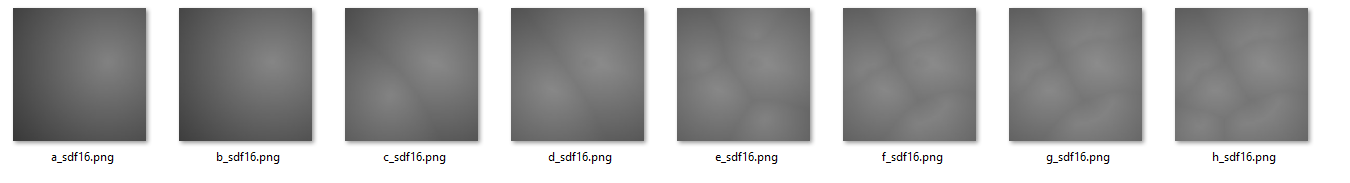
Generated SDFs (scaled, so they appear grayish):
Composited SDF:
wikipedia, Signed distance function, https://en.wikipedia.org/wiki/Signed_distance_function ↩︎
cronrpc, (2025), Signed Distance Field 2D Generator, https://github.com/cronrpc/Signed-Distance-Field-2D-Generator ↩︎
Chris Green. Valve. (2007). Improved Alpha-Tested Magnification for Vector Textures and Special Effects, https://steamcdn-a.akamaihd.net/apps/valve/2007/SIGGRAPH2007_AlphaTestedMagnification.pdf ↩︎
Metric Space, https://en.wikipedia.org/wiki/Metric_space ↩︎
Lisapple, (2017), 8SSEDT , GitHub, https://github.com/Lisapple/8SSEDT ↩︎
Richard Mitton, (2009), Signed Distance Fields, http://www.codersnotes.com/notes/signed-distance-fields/ ↩︎
farteryhr, Correct 8SSEDT, https://replit.com/@farteryhr/Correct8SSEDT#main.cpp ↩︎
蛋白胨, Unity 卡通渲染 程序化天空盒, https://zhuanlan.zhihu.com/p/540692272 ↩︎