Introduction to Perlin Noise
Perlin Noise was developed by Ken Perlin in 1983 for the film Tron as a smooth pseudo-random noise algorithm1. It can generate random patterns with natural-looking texture and is widely used in computer graphics to simulate natural phenomena such as clouds, terrain, fire, wood grain, and water flow2.
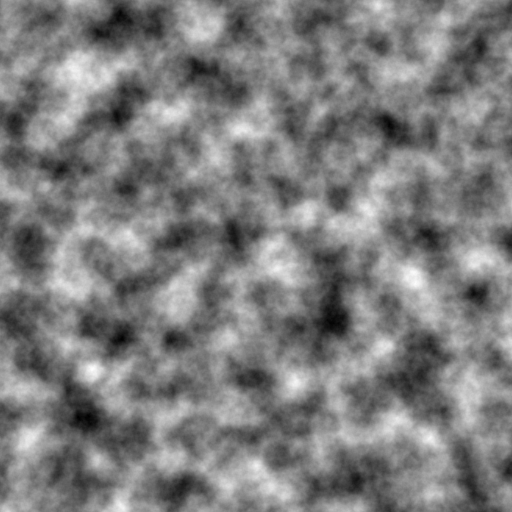
Unlike plain white noise, Perlin Noise has spatial correlation: values at neighboring sample points vary smoothly without abrupt jumps. This smoothness makes the generated textures resemble the continuous variations found in nature.
Minecraft, for example, uses Perlin Noise as a foundational algorithm to generate its effectively infinite world maps.
Types of Noise
1D Uniform White Noise
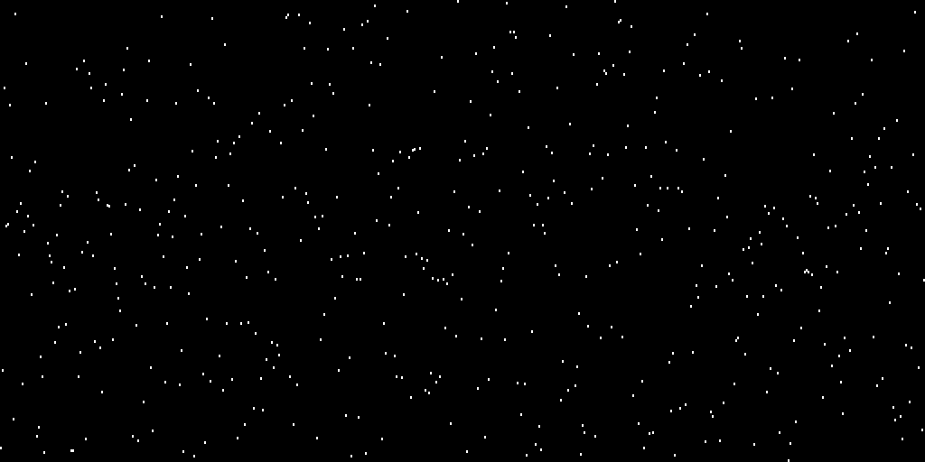
1D uniform white noise is a one-dimensional noise signal where values follow a uniform distribution.
import numpy as np
import matplotlib.pyplot as plt

def sample_random_points(num_points):
    # Sampler function: return num_points random numbers in the range [0, 1)
    return np.random.rand(num_points)

def draw_random_strip_image_from_samples(rand_1d, width, height, filename, thickness=1):
    num_points = len(rand_1d)
    cols_per_point = width // num_points

    rand_pos = (rand_1d * (height - 1)).astype(int)
    img = np.zeros((height, width))
    for i, row in enumerate(rand_pos):
        start_row = max(row - thickness, 0)
        end_row = min(row + thickness + 1, height)
        start_col = i * cols_per_point
        end_col = start_col + cols_per_point
        img[start_row:end_row, start_col:end_col] = 1

    plt.imshow(img, cmap='gray', origin='lower')
    plt.axis('off')
    plt.show()
    plt.imsave(filename, img, cmap='gray')

if __name__ == "__main__":
    rand_noise = sample_random_points(512)
    draw_random_strip_image_from_samples(rand_noise, 1024, 512, "random_noise_1d.png")
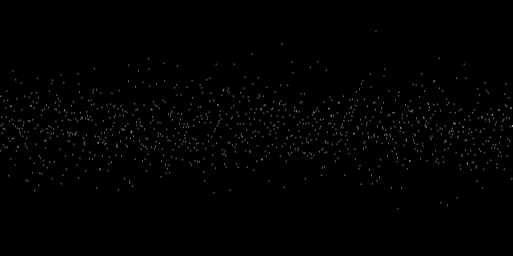
For one-dimensional random noise, the generated points have no correlation between them.
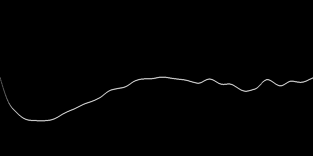
If we use Perlin Noise instead, we get a continuous and smooth curve.
2D Uniform White Noise
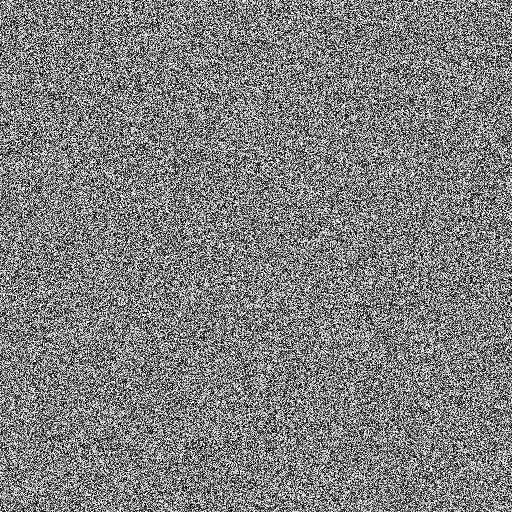
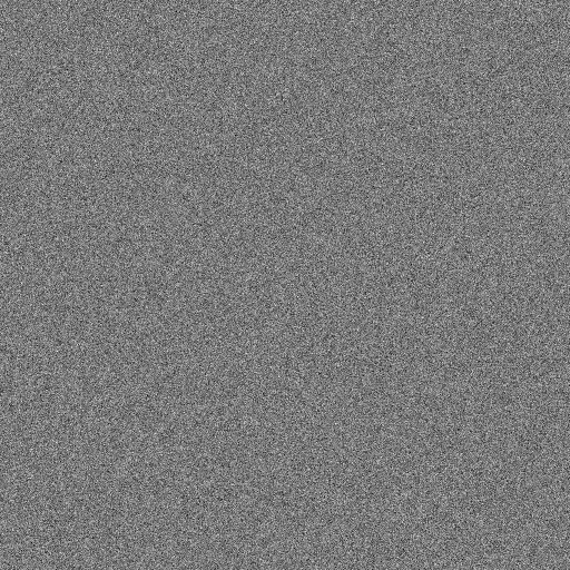
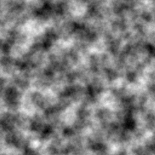
If we randomly generate a noise image with a uniform distribution, the result is uniform white noise: each point has no relation to its neighbors.
import numpy as np
import matplotlib.pyplot as plt

# Generate a 512x512 random floating-point grayscale image with values in [0, 1)
noise = np.random.rand(512, 512)

plt.imshow(noise, cmap='gray')
plt.axis('off')
plt.imsave('random_noise.png', noise, cmap='gray')
Completely random white noise:
Perlin Noise, by contrast, has correlations between neighboring points — adjacent values are required to be close and smooth.
Gaussian White Noise
import numpy as np
import matplotlib.pyplot as plt

# Generate 512x512 Gaussian white noise with mean 0.5 and std deviation 0.1
noise = np.random.normal(loc=0.5, scale=0.1, size=(512, 512))

# Clip values to [0, 1] to avoid display artifacts
noise = np.clip(noise, 0, 1)

plt.imshow(noise, cmap='gray')
plt.axis('off')
plt.imsave('gaussian_white_noise_2d.png', noise, cmap='gray')
plt.show()
Because it is not uniformly distributed, Gaussian noise often looks a bit softer than uniform white noise.
The Gaussian distribution is even more apparent in one dimension, where a clear central band concentrates most of the points.
1D Perlin Noise
To understand the fractal-related concepts in Perlin Noise, we first need to understand the ideas of fade functions, periodicity, and frequency multipliers (octaves)3.
Fade
Given a series of known point values, to estimate values between them we can use linear interpolation to produce straight-line segments or cosine interpolation to produce smooth curves.
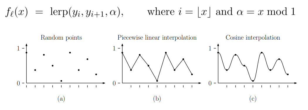
Cosine interpolation can be written as:
$$ x = x1 + (x2-x1) * \frac{1 - \cos(\pi \alpha)}{2} $$
The goal of different interpolation methods is to produce a smooth transition rather than a sharp corner. Besides cosine, cubic, quintic, and other polynomials are commonly used.
Converting linear interpolation into a smooth interpolation like this is called the Fade operation.
In the improved version of his noise algorithm, Perlin used the following Fade function:
$$ t = 6 t^5 - 15 t^4 + 10 t^3 $$
Octaves
If you repeatedly double the sampling frequency, you obtain functions with halved periods. Because doubling frequency corresponds to musical octaves, these levels are called octaves.
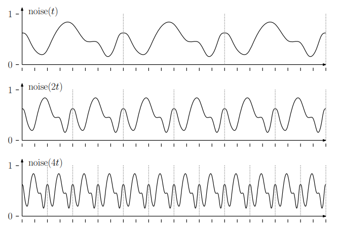
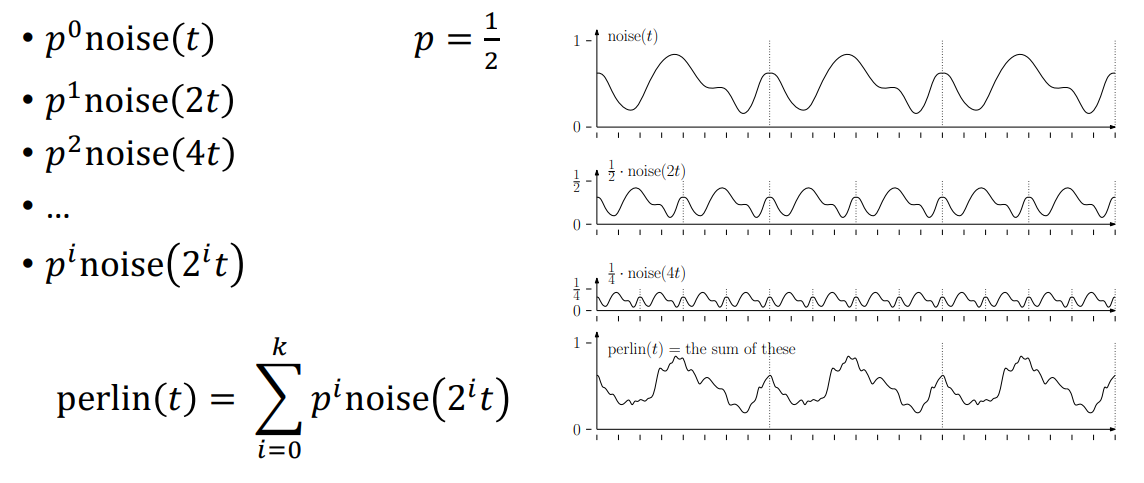
Perlin Noise is composed by mixing noises of different periods with certain weights.
Typically, periods are doubled while weights are halved, which introduces a fractal-like concept.
2D Perlin Noise Generator
Algorithm
Ken Perlin published an implementation of his improved Perlin Noise on his website4.
Perlin Noise is a grid-based gradient noise function commonly used to generate natural-looking textures and terrain. The two-dimensional implementation proceeds as follows:
1. Grid partitioning
Divide the 2D space into a regular integer grid. Each grid corner (lattice point) is associated with a random gradient vector (often unit vectors uniformly distributed in direction).
2. Compute the sample point’s local position
Given a sample point $(x, y)$, determine its containing grid cell by computing the integer coordinates $(X, Y)$ of the cell’s lower-left corner:
$$ X = \lfloor x \rfloor, \quad Y = \lfloor y \rfloor $$
Compute the sample point’s local coordinates relative to the lower-left corner:
$$ x_{\text{rel}} = x - X, \quad y_{\text{rel}} = y - Y $$
3. Compute dot products between corner gradients and displacement vectors
For the four corners of the cell:
$$ (X, Y),\ (X+1, Y),\ (X, Y+1),\ (X+1, Y+1) $$
retrieve each corner’s gradient vector $\vec{g}$ and compute the dot product between $\vec{g}$ and the displacement vector $\vec{d}$ from the corner to the sample point:
$$ \text{dot} = \vec{g} \cdot \vec{d} $$
4. Smooth interpolation
Apply a smooth interpolation function (such as Perlin’s fade) along the $x$ and $y$ axes to bilinearly interpolate the four dot products:
$$ u = \text{fade}(x_{\text{rel}}), \quad v = \text{fade}(y_{\text{rel}}) $$
5. Output noise value
The interpolated result is the noise value at the sample point $(x,y)$, typically in the range approximately $[-1, 1]$.
Python Code
Below is an implementation of 2D Perlin Noise in Python.
import numpy as np
import matplotlib.pyplot as plt
permutation = np.array([ 151,160,137,91,90,15,
131,13,201,95,96,53,194,233,7,225,140,36,103,30,69,142,8,99,37,240,21,10,23,
190, 6,148,247,120,234,75,0,26,197,62,94,252,219,203,117,35,11,32,57,177,33,
88,237,149,56,87,174,20,125,136,171,168, 68,175,74,165,71,134,139,48,27,166,
77,146,158,231,83,111,229,122,60,211,133,230,220,105,92,41,55,46,245,40,244,
102,143,54, 65,25,63,161, 1,216,80,73,209,76,132,187,208, 89,18,169,200,196,
135,130,116,188,159,86,164,100,109,198,173,186, 3,64,52,217,226,250,124,123,
5,202,38,147,118,126,255,82,85,212,207,206,59,227,47,16,58,17,182,189,28,42,
223,183,170,213,119,248,152, 2,44,154,163, 70,221,153,101,155,167, 43,172,9,
129,22,39,253, 19,98,108,110,79,113,224,232,178,185, 112,104,218,246,97,228,
251,34,242,193,238,210,144,12,191,179,162,241, 81,51,145,235,249,14,239,107,
49,192,214, 31,181,199,106,157,184, 84,204,176,115,121,50,45,127, 4,150,254,
138,236,205,93,222,114,67,29,24,72,243,141,128,195,78,66,215,61,156,180
], dtype=np.uint16)
p = np.tile(permutation, 2)
def grad(hash:int, x:float, y:float)->float:
grad_vectors = np.array([
[1, 1], [-1, 1], [1, -1], [-1, -1],
[1, 0], [-1, 0], [0, 1], [0, -1]
])
# Normalize gradient vectors
grad_vectors = grad_vectors / np.linalg.norm(grad_vectors, axis=1)[:, None]
g = grad_vectors[hash % 8]
return np.dot(g, [x, y])
def lerp(t: float, a: float, b: float)->float:
return a + t * (b - a)
def fade(t: float)->float:
return t * t * t * (t * (t * 6 - 15) + 10)
def get_noise(x:float, y:float):
X = int(np.floor(x)) & 255
Y = int(np.floor(y)) & 255
x = x % 1
y = y % 1
u = fade(x)
v = fade(y)
## Here we only need to ensure the hash values are unique
x1 = p[p[X] + Y]
x2 = p[p[X+1] + Y]
x3 = p[p[X] + Y + 1]
x4 = p[p[X+1] + Y + 1]
## x3 x4
## x1 x2
## The direction of each vector is from the integer lattice point towards the noise sample point
return lerp(v, lerp(u, grad(x1, x, y), grad(x2, x - 1, y)),
lerp(u, grad(x3, x, y - 1), grad(x4, x - 1, y - 1)))
def get_perlin_noise(width=256, height=256, scale=8.0, octaves=1, persistence=0.5, lacunarity=2.0):
noise_arr = np.zeros((height, width), dtype=np.float32)
for i in range(height):
for j in range(width):
for k in range(octaves):
x = (j / width) * scale * (lacunarity ** k)
y = (i / height) * scale * (lacunarity ** k)
noise_arr[i, j] += (persistence ** k) * get_noise(x, y)
return noise_arr
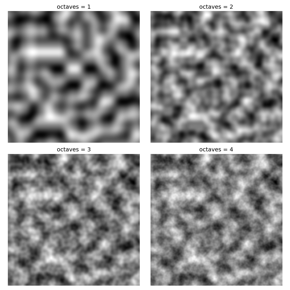
fig, axs = plt.subplots(2, 2, figsize=(10, 10))
for octave_count, ax in zip(range(1, 5), axs.flatten()):
noise_arr = get_perlin_noise(width=256, height=256, scale=8.0, octaves=octave_count)
# Optionally normalize to [0, 1]
noise_arr = (noise_arr - noise_arr.min()) / (noise_arr.max() - noise_arr.min())
ax.imshow(noise_arr, cmap='gray')
ax.set_title(f'octaves = {octave_count}', fontsize=14)
ax.axis('off')
plt.tight_layout()
plt.savefig('perlin_noise_octaves_1_to_4.png')
How to improve gradient values
Using fixed gradient directions instead of gradients produced by a fully uniform random hash helps avoid directional bias that degrades the natural appearance5.
In the original approach, gradient directions were uniformly distributed over the sphere. However, a cube is not a sphere: projections along coordinate axes are shorter while diagonal directions are longer.
This asymmetry in direction can cause a sparse clustering effect: when several nearby gradients that are nearly axis-aligned happen to point the same way, those regions can show anomalously high values.
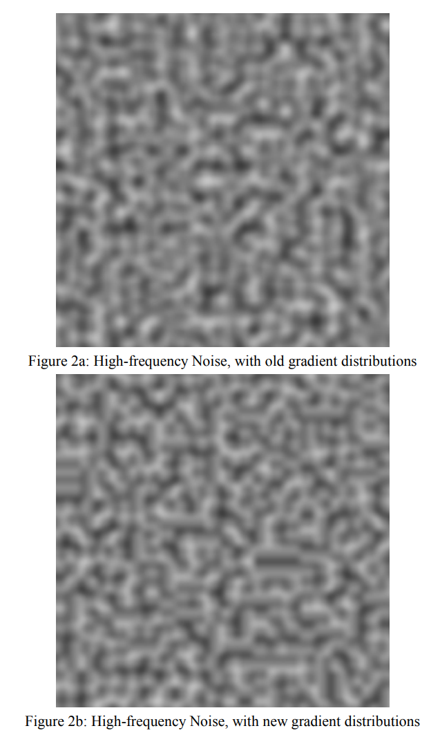
In his improved version, Perlin suggested choosing gradients like:
$$ (1,1,0),(-1,1,0),(1,-1,0),(-1,-1,0), (1,0,1),(-1,0,1),(1,0,-1),(-1,0,-1), (0,1,1),(0,-1,1),(0,1,-1),(0,-1,-1) $$
To avoid the cost of dividing by 12, he expanded the set to 16 directions by adding $(1,1,0),(-1,1,0),(0,-1,1),(0,-1,-1)$.
This article follows that idea: it uses eight planar directions for gradients, and each gradient is normalized to unit length.
For one-dimensional Perlin Noise, you can omit normalization to increase variation. A 1D Perlin Noise can be seen as sampling a 2D Perlin Noise along a line through the lattice; lattice points off the line have zero weight and the result is equivalent to the 1D case. In that situation, the projection of a diagonal gradient onto the horizontal axis is not 1 but $\frac{\sqrt{2}}{2}$.
Improving the Fade function
Perlin5 proposed replacing the fade function with a smoother polynomial (the quintic above).
The reason is: if the second derivative is not smooth, when used to displace surfaces you can see obvious blocky artifacts.
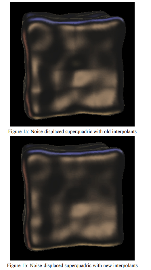
So it’s best to follow these principles:
- At 0 and 1, derivatives should be 0 so transitions are as smooth as possible. Higher-order derivatives can also be made zero.
- $ f(0) = 0 $
- $ f(1) = 1 $
Examples / Applications
Python Noise Library
In practice, you rarely need to implement Perlin Noise from scratch — the Python noise library can generate Perlin Noise directly.
import numpy as np
import matplotlib.pyplot as plt
from noise import pnoise2

width, height = 512, 512
scale = 64.0  # Controls the "stretch" of the noise; larger values make changes occur more slowly
octaves = 6
persistence = 0.5
lacunarity = 2.0

noise = np.zeros((height, width))
for y in range(height):
    for x in range(width):
        nx = x / scale
        ny = y / scale
        noise[y][x] = pnoise2(nx, ny, octaves=octaves, persistence=persistence, lacunarity=lacunarity, repeatx=1024, repeaty=1024, base=0)

# Perlin noise is typically in approximately [-1, 1]; normalize to [0, 1]
noise = (noise - noise.min()) / (noise.max() - noise.min())

plt.imshow(noise, cmap='gray')
plt.axis('off')
plt.imsave('perlin_noise_2d_lib.png', noise, cmap='gray')
plt.show()
Because it is optimized, generation is very fast:
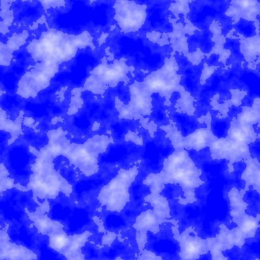
Clouds
Use Perlin Noise to simulate simple cloud textures.
- Simulate the dissipating edges of clouds.
- Simulate central highlights; above a threshold, values remain unchanged, and within a certain range apply the following operation:
$$ \text{Intensity} = \max(\text{Intensity} - 40, 0) $$
import numpy as np
from PIL import Image

# Read grayscale image, keep integer values in 0~255
img = Image.open('perlin_noise_2d_lib.png').convert('L')
arr = np.array(img).astype(np.int32)  # 0~255

height, width = arr.shape

# Create an RGB image, pure blue background (R,G,B) = (0,0,255)
rgb_img = np.zeros((height, width, 3), dtype=np.uint8)
for y in range(height):
    for x in range(width):
        r, g, b = 0, 0, 255

        cloud_intensity = arr[y, x]  # 0~255

        cloud_intensity = cloud_intensity - 30

        if cloud_intensity < 100:
            cloud_intensity = max(cloud_intensity - 40, 0)

        # Linear blend: cloud_intensity represents white cloud strength (0~255)
        # Compute weight: cloud_intensity / 255
        w = cloud_intensity / 255

        r = int(r * (1 - w) + w * 255)
        g = int(g * (1 - w) + w * 255)
        b = int(b * (1 - w) + w * 255)

        rgb_img[y, x, 0] = r
        rgb_img[y, x, 1] = g
        rgb_img[y, x, 2] = b

# Save the uint8 array directly
im = Image.fromarray(rgb_img)
im.save('perlin_cloud.png')
Cloud result:
Unity Noise Editor
After installing the Terrain Tools package in Unity, you can find the noise generator under Window > Terrain > Edit Noise. It allows you to directly generate various types of noise, including Perlin Noise, and export them as textures.
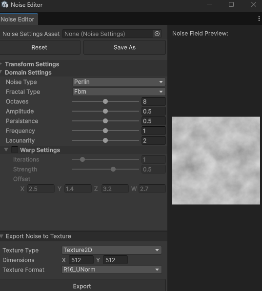
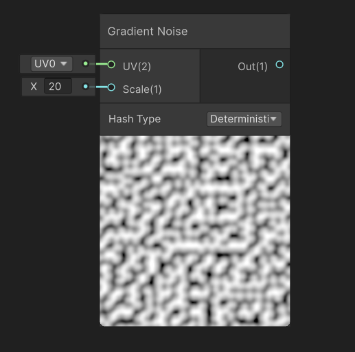
Or, you can also directly find Gradient Noise in Unity Shader Graph.
Perlin, K. (1985). An image synthesizer. ACM Siggraph Computer Graphics, 19(3), 287-296. ↩︎
Perlin Noise wiki, https://en.wikipedia.org/wiki/Perlin_noise ↩︎
Roger Eastman. (2019). CMSC425.01 Spring 2019 Lecture 20: Perlin noise I. University of Maryland. https://www.cs.umd.edu/class/spring2019/cmsc425/handouts/CMSC425Day20.pdf ↩︎
Ken Perlin. (2022). Improved Noise reference implementation. https://mrl.cs.nyu.edu/~perlin/noise/ ↩︎
Perlin, K. (2002, July). Improving noise. In Proceedings of the 29th annual conference on Computer graphics and interactive techniques (pp. 681-682). ↩︎ ↩︎