This article focuses solely on the following topics:
- Transition from trigonometric series expansion to the Euler form of the Fourier transform
- What the Discrete Fourier Transform is
- What the 2D Fourier Transform is
- Explanation of the 2D Discrete Fourier Transform from the 2D Fourier Transform
- How to perform a 2D Fourier transform on an image
- Periodicity issues in the 2D Fourier transform
- Understanding the centering of the 2D frequency spectrum from the periodicity of the 2D Fourier transform
Fourier Series
A Fourier series is a mathematical tool that represents a periodic function as an infinite sum of sines and cosines.
Trigonometric Series Expansion
The Fourier transform was originally based on the trigonometric series expansion: a periodic function can be expressed as a linear combination of sine and cosine functions:
$$ f(t) = a_0 + \sum_{n=1}^{\infty} a_n \cos(n\omega_0 t) + b_n \sin(n\omega_0 t) $$
where $\omega_0 = \frac{2\pi}{T}$ is the fundamental frequency.
Complex Exponential Form
Using Euler’s formulas:
$$ \cos(x) = \frac{e^{ix} + e^{-ix}}{2}, \quad \sin(x) = \frac{e^{ix} - e^{-ix}}{2i} $$
the Fourier series can be rewritten in the complex exponential form:
$$ f(t) = \sum_{n=-\infty}^{\infty} c_n e^{in\omega_0 t} $$
where $c_n$ are complex coefficients that encapsulate both sine and cosine information. The Euler form is more symmetric and easier to manipulate, and it lays the foundation for generalizing to continuous and multidimensional cases.
Here, the index $n$ runs from $-\infty$ to $\infty$.
Discrete Fourier Transform (DFT)
The Discrete Fourier Transform is a crucial branch of Fourier analysis. It converts a finite-length discrete signal (typically digital) from the time or spatial domain into the frequency domain, representing it as a sum of complex frequency components.
In practice, we work with finite, discrete data. The DFT is defined as:
$$ X[k] = \sum_{n=0}^{N-1} x[n] \cdot e^{-i \frac{2\pi}{N}kn}, \quad k = 0, 1, \dots, N-1 $$
The corresponding inverse transform is:
$$ x[n] = \frac{1}{N} \sum_{k=0}^{N-1} X[k] \cdot e^{i \frac{2\pi}{N}kn} $$
The DFT maps the time-domain signal $x[n]$ to the frequency-domain $X[k]$, where each $X[k]$ corresponds to the amplitude and phase of a specific frequency component.
Negative Frequencies and Periodic Reordering
In the DFT, negative frequencies naturally arise.
Although the DFT index $k$ is a non-negative integer, the Fourier frequencies exhibit periodicity modulo $N$:
$$ e^{-i \frac{2\pi}{N} k n} = e^{-i \frac{2\pi}{N} (k + mN) n}, \quad \forall m \in \mathbb{Z} $$
Thus, frequency $k = N - 1$ is equivalent to $-1$, $k = N - 2$ to $-2$, and so on.
We can reinterpret the frequency indices to span from negative to positive frequencies:
$$ k = -\frac{N}{2}, \dots, -1, 0, 1, \dots, \frac{N}{2} - 1 \quad (\text{for even } N) $$
By reordering (or centering) the spectrum, the result aligns more intuitively with symmetric positive and negative frequency components.
After applying a 2D Fourier transform to an image, we often center the spectrum so that low-frequency components appear at the center.
2D Fourier Transform
The Fourier transform can be extended from the 1D case to 2D.
What Is the 2D Fourier Transform?
The continuous 2D Fourier transform of a function $f(x, y)$ is defined as:
$$ F(u, v) = \iint_{-\infty}^{\infty} f(x, y) \cdot e^{-i2\pi (ux + vy)} , dx,dy $$
Its inverse is:
$$ f(x, y) = \iint_{-\infty}^{\infty} F(u, v) \cdot e^{i2\pi (ux + vy)} , du,dv $$
Here, $(x, y)$ are spatial-domain coordinates and $(u, v)$ are frequency-domain coordinates. The transform $F(u, v)$ describes the amplitude and phase of each frequency component in the signal.
2D Discrete Fourier Transform
For a discrete $M \times N$ function $f[m, n]$, the 2D DFT is defined as:
$$ F[k, l] = \sum_{m=0}^{M-1} \sum_{n=0}^{N-1} f[m, n] \cdot e^{-i 2\pi \left( \frac{km}{M} + \frac{ln}{N} \right)} $$
The inverse 2D DFT is:
$$ f[m, n] = \frac{1}{MN} \sum_{k=0}^{M-1} \sum_{l=0}^{N-1} F[k, l] \cdot e^{i 2\pi \left( \frac{km}{M} + \frac{ln}{N} \right)} $$
Periodicity of the 2D Fourier Transform
Like the 1D DFT, the 2D DFT is periodic:
$$ F[k + M, l] = F[k, l], \quad F[k, l + N] = F[k, l] $$
This means the spectrum repeats in both horizontal and vertical directions.
The frequency indices $k$ and $l$ range from $0$ to $M-1$ and $0$ to $N-1$, but these indices are understood modulo the respective dimensions. For example, when $k > \tfrac{M}{2}$, the actual frequency corresponds to the negative frequency $k - M$. The same applies for $l > \tfrac{N}{2}$.
How to Perform a 2D Fourier Transform on an Image
In Python, libraries like NumPy or OpenCV make it easy to compute a 2D Fourier transform. For example, using NumPy:
import numpy as np
import matplotlib.pyplot as plt
from PIL import Image

# Load and convert the image to grayscale
img = Image.open('doge.jpg').convert('L')
f = np.array(img)

# Compute the 2D Fourier transform
F = np.fft.fft2(f)

# Magnitude and phase spectra
magnitude_spectrum = np.abs(F)
phase_spectrum = np.angle(F)
log_magnitude = np.log(1 + magnitude_spectrum)

# Create subplots
fig, axs = plt.subplots(1, 3, figsize=(15, 5))

# Original image
axs[0].imshow(f, cmap='gray')
axs[0].set_title('Original Image')
axs[0].axis('off')

# Magnitude spectrum
axs[1].imshow(log_magnitude, cmap='gray')
axs[1].set_title('Magnitude Spectrum (log)')
axs[1].axis('off')

# Phase spectrum
im = axs[2].imshow(phase_spectrum, cmap='gray')
axs[2].set_title('Phase Spectrum')
axs[2].axis('off')

# Add a colorbar to the phase spectrum
fig.colorbar(im, ax=axs[2], shrink=0.7)

plt.tight_layout()
plt.show()
After running this, you will see the magnitude and phase spectra:
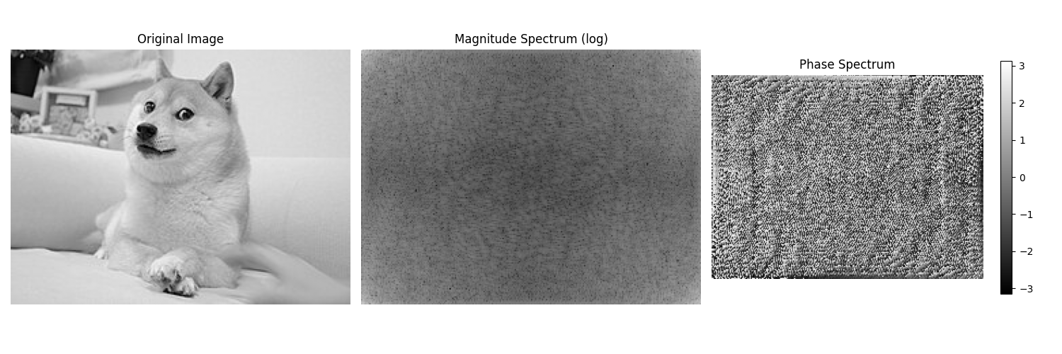
Inverse Transform to Recover the Image (Magnitude + Phase)
The Fourier transform results are complex, containing magnitude and phase information. Retaining only one of them is insufficient to reconstruct the original image.
To recover the image:
import numpy as np
import matplotlib.pyplot as plt
from PIL import Image
# Load and convert the image to grayscale
img = Image.open('doge.jpg').convert('L')
f = np.array(img)
# Compute the 2D Fourier transform
F = np.fft.fft2(f)
# Perform the inverse Fourier transform
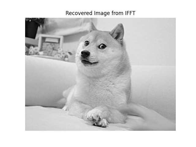
recovered = np.fft.ifft2(F)
recovered_real = np.real(recovered)
plt.imshow(recovered_real, cmap='gray')
plt.title('Recovered Image from IFFT')
plt.axis('off')
plt.show()
The reconstructed image should match the original.
Centering the Spectrum
To observe the frequency distribution more clearly, we often center the spectrum so that low frequencies are in the middle and high frequencies are around the edges.
You can use np.fft.fftshift to center the spectrum:
import cv2
import numpy as np
import matplotlib.pyplot as plt

img = cv2.imread('doge.jpg', cv2.IMREAD_GRAYSCALE)

f = np.fft.fft2(img)

fshift = np.fft.fftshift(f)

magnitude_spectrum = 20 * np.log(np.abs(fshift) + 1)

plt.figure(figsize=(12, 6))
plt.subplot(1, 2, 1)
plt.title('Original Image')
plt.imshow(img, cmap='gray')

plt.subplot(1, 2, 2)
plt.title('Magnitude Spectrum')
plt.imshow(magnitude_spectrum, cmap='gray')

plt.show()
After centering, the low-frequency components move to the center, making it easier to observe textures and directional patterns.

High-level contours are represented by the low-frequency center, while fine details and textures are captured by the high-frequency components at the edges.